

This blog series is part of the joint collaboration between Canonical and Manceps. Part 1 is here.
Introduction
Kubeflow Pipelines is a great way to build portable, scalable machine learning workflows. It is a part of the Kubeflow project that aims to reduce the complexity and time involved with training and deploying machine learning models at scale.
In Part 2 of this blog series, you will work on building your first Kubeflow Pipelines workflow as you gain an understanding of how it’s used to deploy reusable and reproducible ML pipelines. 🚀
In Part 1, we covered WHY Kubeflow brings the right standardization to data science workflows. Now, let’s see HOW you can accomplish that with Kubeflow Pipelines.
Let’s get our hands dirty! 👨🏻🔬
Building your first Kubeflow pipeline
In this experiment we will use the Basic classification with Tensorflow example to build our first Kubeflow Pipeline. You can follow the process of migration into the pipeline using this Jupyter Notebook.
Ready? 🚀
Step 1: Deploy Kubeflow and access the dashboard
If you haven’t had the opportunity to launch Kubeflow, don’t worry! You can deploy Kubeflow easily using Microk8s by following the tutorial - Deploy Kubeflow on Ubuntu, Windows and MacOS.
We recommend deploying Kubeflow on a system with 16GB of RAM or more. Otherwise, spin-up a virtual machine instance somewhere with these resources (e.g. t2.xlarge EC2 instance) and follow the same steps.
You can find alternative deployment options here.
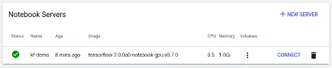
Step 2: Launch notebook server
Once you have access to the Kubeflow dashboard, setting up a jupyter notebook server is fairly straightforward, just follow the steps here.
Step 3: Git clone our example notebook
Once in the Notebook server, launch a new terminal from the menu on the right (New > Terminal).
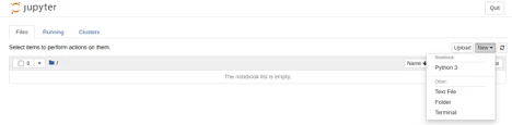
In the terminal, download this Notebook from GitHub:
Now, open the “KF_Fashion_MNIST” notebook:
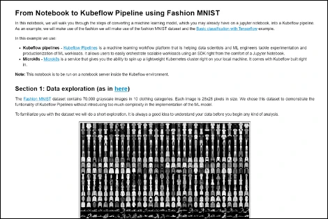
Jupyter notebook for this experiment - here.
Step 4: Initiate Kubeflow Pipelines SDK
Now that we’re on the same page, we can kickstart our project together in the browser. As you see, the first section is adapted from the Basic classification with Tensorflow example. Let’s skip that and get on with converting this model into a running pipeline.
To ensure access to the packages needed through your Jupyter Notebook instance, begin by installing Kubeflow Pipelines SDK (kfp) in the current userspace:
Step 5: Convert Python functions to container components
The Kubeflow Python SDK allows you to build lightweight components by defining python functions and converting them using func_to_container_0p.
To package your python code inside containers, you define a standard python function that contains a logical step in your pipeline. In this case, we have defined two functions: train and predict.
The train component will train, evaluate, and save your model.
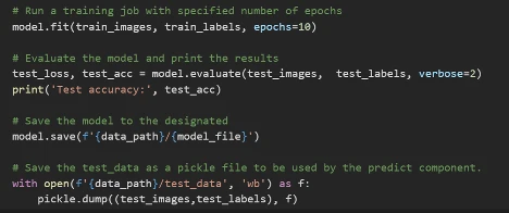
The predict component takes the model and makes a prediction on an image from the test dataset.
The code used in these components is in the second part of the Basic classification with Tensorflow example, in the “Build the model” section.
The final step in this section is to transform these functions into container components. You can do this with the func_to_container_op method as follows.
Step 6: Define Kubeflow Pipeline
Kubeflow uses Kubernetes resources which are defined using YAML templates. Kubeflow Pipelines SDK allows you to define how your code is run, without having to manually manipulate YAML files.
At compile time, Kubeflow creates a compressed YAML file which defines your pipeline. This file can later be reused or shared, making the pipeline both scalable and reproducible.
Start by initiating a Kubeflow client that contains client libraries for the Kubeflow Pipelines API, allowing you to further create experiments and runs within those experiments from the Jupyter notebook.
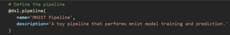
Define the pipeline name and description which will be visualized on the Kubeflow dashboard
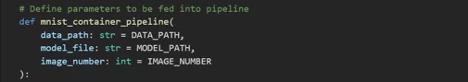
Next, define the pipeline by adding the arguments that will be fed into it.
In this case, define the path for where data will be written, the file where the model is to be stored, and an integer representing the index of an image in the test dataset:
Step 7: Create persistent volume
One additional concept that is important to understand is the concept of Persistent Volumes. Without adding persistent volumes, all of the data would be lost if the notebook was terminated for any reason. The Kubeflow Pipelines SDK allows for the creation of persistent volumes using the VolumeOp object.
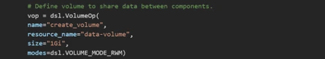
VolumeOp parameters include:
- name - the name displayed for the volume creation operation in the UI
- resource_name - name which can be referenced by other resources.
- size - size of the volume claim
- modes - access mode for the volume (See Kubernetes docs for more details on access mode).
Step 8: Define pipeline component
It is now time to define your pipeline components and dependencies. We do this with ContainerOp, an object that defines a pipeline component from a container.
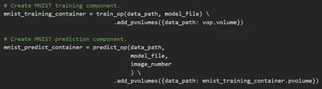
The train_op and predict_op components take arguments which were declared in the original python function. At the end of the function we attach our VolumeOp with a dictionary of paths and associated Persistent Volumes to be mounted to the container before execution.
Notice that while train_op is using the vop.volume value in the pvolumes dictionary, the <Container_Op>.pvolume argument used by the other components ensures that the volume from the previous ContainerOp is used, rather than creating a new one.
This inherently tells Kubeflow about our intended order of operations. Consequently, Kubeflow will only mount that volume once the previous <Container_Op> has completed execution.
The final print_prediction component is defined somewhat differently. Here we define a container to be used and add arguments to be executed at runtime.
This is done by directly using the ContainerOp object.
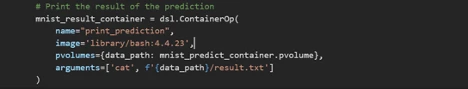
ContainerOp parameters include:
- name - the name displayed for the component execution during runtime.
- image - image tag for the Docker container to be used.
- pvolumes - dictionary of paths and associated Persistent Volumes to be mounted to the container before execution.
- arguments - command to be run by the container at runtime.
Step 8: Compile and run
Finally, this notebook compiles your pipeline code and runs it within an experiment. The name of the run and of the experiment (a group of runs) is specified in the notebook and then presented in the Kubeflow dashboard. You can now view your pipeline running in the Kubeflow Pipelines UI by clicking on the notebook link run.
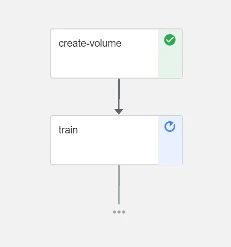
Results
Now that the pipeline has been created and set to run, it is time to check out the results. Navigate to the Kubeflow Pipelines dashboard by clicking on the notebook link run or Pipelines → Experiments → fasion_mnist_kubeflow. The components defined in the pipeline will be displayed. As they complete the path of the data pipeline will be updated.
To see the details for a component, click directly on the component and dig into a few tabs. Click on the logs tab to see the logs generated while running the component.
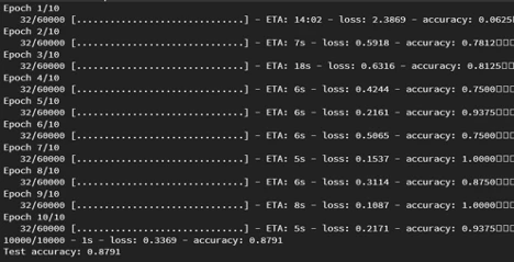
Once the echo_result component finishes executing, you can check the result by observing the logs for that component. It will display the class of the image being predicted, the confidence of the model on its prediction, and the actual label for the image.
Final Thoughts
Kubeflow and Kubeflow Pipelines promise to revolutionize the way data science and operations teams handle machine learning operations (MLOps) and pipelines workflows. However, this fast-evolving technology can be challenging to keep up with.
In this blog series we went through a conceptual overview, in part 1, and a hands-on demonstration in part 2. We hope this will get you started on your road to faster development, easier experimentation, and convenient sharing between data science and DevOps teams.
To keep on learning and experimenting with Kubeflow and Kubeflow Pipelines:
- Play with Kubeflow examples on GitHub
- Read our overview here
- Visit ubuntu.com/kubeflow
← Go Back to Part 1